Is It A Viola? A CNN-Based Violin-Viola Binary Classifier

July 30, 2025

The viola and violin are two members of the violin family of string instruments, which consist of bowed four-stringed instruments. Both instruments share three strings, G3, D4, A4, but the violin has a high E5, while the viola has a low C3. The viola’s lower range naturally lends itself to be slightly bigger, but still played on-the-shoulder. However, with this selection of strings comes acoustic imperfection — if we wanted the viola’s sound to resonate perfectly, we would demand that the viola be substantially larger than it is now, which would compromise its playing technique (In fact, this has led to the creation of the “vertical viola,” which maintains the pitches of the standard viola, but allows it to be much larger, and played in the same manner as the cello)¹. This quality results in the viola sounding mellower than the more brilliant-sounding violin, which is sized perfectly for its strings. Hence, sharp-eared individuals will be able to tell a violin from a viola, even when both are playing the exact same pitches. This is the key to differentiating the two instruments, but it is a subtle one. Without knowledge of the piece being performed, even for those familiar with the sound of both violin and viola may find the task of identifying which instrument is being performed to be difficult.

This yields the question — can a machine learning model do it?

Prior Work

The task of instrument classification is not new. Many different teams have researched models, ranging for mel spectrogram Convolutional Neural Networks (CNN)² to mel-frequency cepstral coefficients Support Vector Machines (SVM)³ to statistical models on features such as highest and lowest pitch⁴. But most of these models have been on instruments which significantly different timbre and sound quality, such as telling apart violin and clarinet. As far as I could find, only one paper exists exploring classification between these two similar-sounding instruments⁴, and using a random forest model on statistical features, they achieved 94% accuracy on a dataset of solo violin and solo viola music throughout all historical eras. Notably, their model outperforms their designed CNN quite significantly.

However, training on their same dataset (ignoring historical eras), I have achieved equivalent accuracy (~94%) using a CNN, using a non-square kernel and implementing a variant of SpecAugment++⁵, a data augmentation technique. In the rest of this post, I will explain all the CNN variants and data augmentation I tried.

Dataset

The paper⁴ puts together both a training and testing set of solo violin and solo viola pieces, separated by era, i.e. baroque, classical, romantic, and modern. Some of the viola pieces were originally written for viola, some are violin pieces transposed for viola (e.g. Paganini caprices) and some are cello pieces written up an octave for viola (e.g. Bach suites). I have taken these datasets and disregarded their era, considering only their instrument. Additionally, I divide the test set into two equal parts, making one a test set and the other a validation set. This split is not fixed, as it happens after the data preprocessing without a fixed seed.

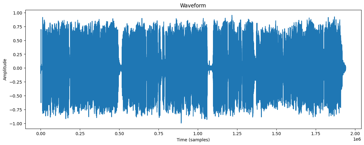
While the initial dataset consists entirely of audio files, as suggested before, there are several ways to process these audio files. An audio file, fundamentally, is a waveform, samples of the air pressure sampled at a constant rate per second. For our data, it was 44,100 samples per second.

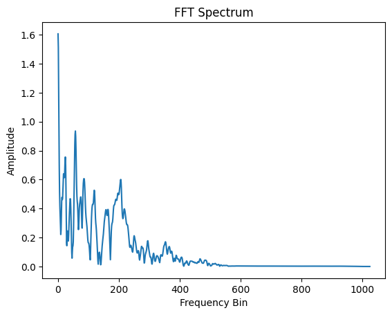
Using the fast Fourier transform, we decompose a range of these samples into their underlying sine functions, and, instead of plotting amplitude vs time, we plot magnitude of the frequency against the frequency itself.

This is not a spectrogram yet. To create the spectrogram, we calculate the FFT on short overlapping time segments. This is known as the short-time Fourier transform, we may now plot these as frequency vs time, alongside a color spectrum. The brighter the color, the greater the magnitude of that particular frequency at that particular time. I used the default settings of the librosa Python library, which calculates FFT over 2048 samples, offset by 512 samples each time.

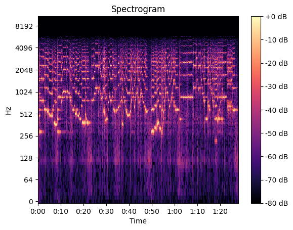
This is the spectrogram. But recall that I used the mel spectrogram⁶. What does that mean? Studies have shown that humans do not hear pitch linearly, but in fact closer to a nonlinear scale called the mel scale. We simply convert our frequency scale to use this scale instead.

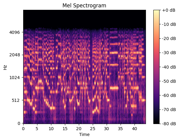
To prepare the data, I divided each .wav file into segments of length 6 seconds, offset by 2 seconds each. For instance, a 14 second audio file would yield 5 spectrograms, each of length 6 seconds. The spectrogram, using standard librosa calculations, ends up having 128 frequency channels over 517 timestamps. The decision to divide each recording up was made so as to greatly increase the number of samples available, and also to create a standard image size to convolve over.

Model

In Tamanna et al. (2024)², which is on five-instrument classification, after performing hyperparameter optimization, they find that the ideal CNN has the following layers.

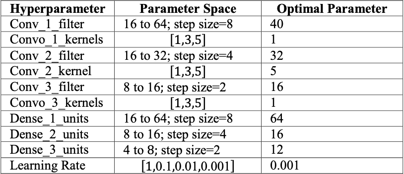
This yielded them an accuracy of ~86%. Certainly a fine starting point, so I also started here.
Initially, I found that the instruments were too similar, and training set imbalance too wide for the standard cross-entropy loss to work properly, as it resulted in the model simply always choosing violin. I tested around with some weights, and discovered that \((1.0, 1.2)\) on (vln, vla) respectively resulted in a loss function that properly balanced the two classes.

Once I had figured out my loss function woes, I found that this model yielded me approximately 86% on the test set, same as the paper. I endeavored to improve this.

Kernel Size

My real innovation, my actual improvement on CNN for instrument classification, came in a decision I made regarding the kernel size. Every prior paper I found accepted a square kernel, but I question this tacit assumption. Certainly, temporal effects matter in determining instrument, but the Acoustical Society of America claims that “timbre depends primarily upon the frequency spectrum.” What if we instead invested entirely in frequency, at least for the first layer?

Hence, I (rather arbitrarily — I am aware that the proper way of testing this should have been cross-validation along different parameters. This work is not finished, and I likely will return and properly find the best parameters to use) decided that the first layer of the kernel should have size \((5,1)\) with stride \((2,1)\). The second layer returns the stride to \(1\), but maintains another rectangular kernel of size \((3,2)\) in order to incorporate some temporal effects, with Dropout in between these first two layers for good measure.

This innovation saw substantial improvement, with test accuracy of 93%, with recall \(0.92\), precision \(0.92\), and F1 score \(0.92\).

Augmentation

Instead of hyperparameter optimization, I sought to create a more robust model through data augmentation. The paper which used the architecture I initially started with applied the CutMix algorithm, so I started there as well.

CutMix

The CutMix algorithm⁷, intuitively, replaces a random rectangular cutout of one training example, and replaces it with the same region in another training example. It also mixes the labels, according to the ratio of example 1 to example 2.

Mathematically, let \(x_1, x_2\in\mathbb{R}^{W\times H}\) be training images with labels \((y_1,y_2)\in\{0,1\}.\) We seek the augmented training sample \(x',y'\) where

and

where \(\mathbf{M}\in\{0,1\}^{W\times H}\) is a binary mask, and \(\lambda\) is the ratio between \(x_2\) and \(x_2\) in the augmented image. We sample \(\lambda\sim\text{Unif}(0,1),\) which we then use to sample the bounding box \(\mathbb{B}\) that determines \(\mathbb{M}.\)

We represent

where

and

This results in the ratio of bounding box to image size \(\frac{wh}{WH}=\sqrt{1-\lambda}.\) Then, we define the mask \(\mathbf{M}\) by

To run the augmentation technique, we randomly select two training examples within each batch and perform the above operations.

Results wise, this yielded a test accuracy of ~%92, which is actually slightly worse than the prior model. I would imagine this is due the similarities in timbre between violin and viola, so the mixed labels does not really create any more robustness than not using it. I realized that I needed to try a different technique.

MixUp

On the PyTorch tutorial for implementing CutMix, it also describes randomly choosing between CutMix and MixUp. This led me to try both pure MixUp and that same random choice for any two sampled examples. But first, what MixUp is.⁸

MixUp is actually significantly simpler than CutMix, because it is only defined by one random parameter instead of five. We sample \(\lambda\sim\text{Unif}(0,1),\) and then, given two random training examples \(x_1,x_2\) with labels \(y_1,y_2,\) we let

and

To clarify this means, for \(0\leq i\leq W\) and \(0\leq j\leq H\), we let

where \(x^{(ij)}\) represents the pixel at \((i,j)\).

Random choice between CutMix and MixUp, did not fare particularly much better than the base model, with test accuracy of ~93%, but MixUp alone did show good improvement with a test accuracy of ~94%, albeit with recall \(0.91\), precision \(0.94\), and F1 score \(0.92\). So far, MixUp has yielded the best results!

SpecAugment

It’s at this point I went looking for data augmentation specifically designed for spectrograms. While MixUp remained effective, spectrograms are more structured, and for my purposes, one axis may be more relevant than the other, while with traditional images this is usually not the case. In my search, I found SpecAugment.⁹

However, the design of SpecAugment is essentially just Cutout, except hiding entire frequency rows and time columns, and sometimes replacing them with random noise. I did not feel particularly drawn towards trying this method, but that’s when I found SpecAugment++.

SpecAugment++

Designed as an improvement to SpecAugment, applies masking with some probability on the hidden states.⁵ In implementation, this requires a layer. I only used Mixture Masking, whose design is as follows:

Given two 2D hidden state \(h_1,h_2\) with width \(W\) and height \(H\), we sample

and

Then, we get the new hidden state:

Since this augmentation method is applied directly as a layer, we in fact take \(h_1\) as the “base” example, and then sample \(h_2\) from the rest of the batch. Then, we replace \(h_1\) with the augmented sample.

In my own design, I applied Mixture Masking with probability \(\frac{3}{5}\) at the start, between the first and second layers, and between the second and third layers.

I would also like to note that because SpecAugment++ is not a particularly well-known paper, the technique has not been implemented natively within any libraries. Therefore, I implemented Mixture Masking myself.

With just Mixture Masking, I got the best results of all. A test accuracy of nearly ~95%, with recall nearing \(0.95\), precision nearing \(0.94\), and F1 score of \(0.94\). By far, this is the best model I could use. I did try mixing Mixture Masking with MixUp (as well as CutMix, and both at the same time), but it did not lead to any great improvements.

Accessing the Model

Instead of leaving this model inside a Jupyter Notebook and a .pth file, I decided that I wanted to make it more easily accessible. Hence, I decided to improve my webdev abilities and create a frontend and a backend for this. By no means is either particularly fleshed out, and I decided to use Streamlit for the frontend and FastAPI for the backend, two Python libraries.

At a high level, the webpage itself simply has a file uploader, which only accepts audio files (i.e. .mp3, .wav, and .m4a files). It ships those files off to the API, which preprocesses it by splitting it into segments of 6 seconds, offset by 2 (as before) and getting their mel spectrograms. These are then fed into the model, which returns the class probabilities. I average the probabilities over all the six-second segments, and then return those averaged probabilities. The frontend displays these probabilities, as well as the \(\arg\max\) of them.

Reflection and Next Steps

I tested these on a few random YouTube videos that I confirmed did not exist in the train or test set, as well as recordings of myself playing viola! It got all the YouTube videos correct (which was very exciting!), but for some reason was really sure that I personally am a violinist, which is a personal tragedy and tells me that I need to try out different architectures. My hypothesis is that my viola has always sounded less mellow and more brilliant than most violas, and I myself have found that my tone is much different when I borrow my friends’ instruments.

I’m really glad that I decided to do some engineering. A lot of the ML projects on my GitHub simply live in Python files and notebooks, and it felt good to get some more practice with SWE. I’ve done very little work with backend, and just in reading about how to use FastAPI, I learned much more about backend design than the actual code I used would imply. Streamlit, on the other hand, is much more akin to a prototype frontend, and maybe in the future I’ll build a proper frontend, but this is comparatively lower on my priority list.

There are several other non-neural net architectures that I would like to try. As mentioned before, others have trained support vector machines on mel-frequency cepstral coefficients and other frequency-type statistics. I would like to implement some of those, and then quite possibly train an ensemble using the best of those models and the CNN described in this blog post.

The code from this project may be found here.

Bibliography